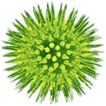
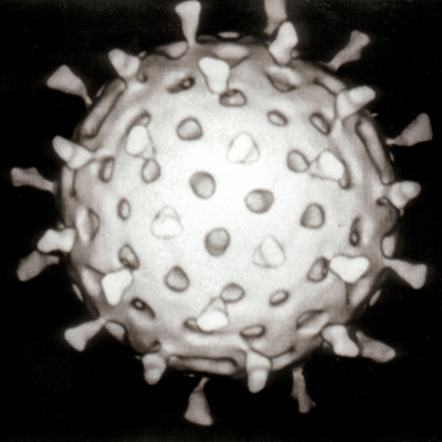
Rotavirus as seen in an electron microscope, reconstructed by computer [image source].
Some things are too small to see. Microscopes help us to zoom in on some of them, but only up to a point. Objects smaller than a few hundred nanometers don’t even reflect visible light: a 1,000,000× magnifying glass wouldn’t be able to show us anything, despite its magnification strength. To study the shapes of things smaller than this, scientists bounce electrons (or other particles) off of them, but this technique is a bit more like sonar than sight.
To be specific, concepts such as color have no meaning for objects this small. Color is the pattern of wavelengths of light that a substance likes to reflect— for instance, grass absorbs red light (570–750 nm) and blue light (380–495 nm) but reflects green (495–570 nm). A strawberry reflects red but absorbs green and blue. Most viruses are between 20 and 300 nm, smaller than all visible wavelengths, so they don’t reflect much visible light. They are without color in a more fundamental sense than something that is merely gray.
This may cause consternation for virologists who want to explain what the critters look like, but it derives from a deep principle of physics that relates to the bandwidths of radio stations, the Heisenberg Uncertainty Principle, and why you can put staples in the microwave.
Visible light is a human-centric term. Electromagnetic waves can have any wavelength, but our eyes are only sensitive to a range from about 380 nm to about 750 nm, a factor of two. In music, a factor of two difference in the wavelengths of sound waves is an octave, so one could say that humans see an octave of light. However, human hearing is sensitive to many distinct semitones between middle C and high C, whereas our vision can only distinguish three “notes”: red, green, and blue. Secondary colors and mixtures (e.g. ochre, burnt sienna, and fuchsia) are analogous to musical chords, not pure pitches.
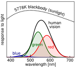
Response of the three types of light-sensitive cells in human eyes.
The range of visible light is not sharply defined, either. Human eyes have three types of light-sensitive cells— red, green, and blue cone cells— which respond to broad, overlapping ranges of wavelengths. Red and green largely overlap; red light looks different from green light only because the red cone cells respond to it slightly more than the green cone cells (a stronger signal is sent to the brain, and the brain sorts it out). Individual humans have different response curves, too. Some people’s red and green sensitivities overlap so completely that they are red-green colorblind.
There’s even more variation in the animal kingdom. Dogs and cats have only two kinds of cone cells, sensitive to green and blue. They might notice motion on your red-green-blue computer monitor, which was tuned for human eyes, but the colors wouldn’t make sense to them. Horses see red and blue. Birds see four primary colors, one of which is ultraviolet— shorter wavelengths than 380 nm. They might be able to see a magnified image of a virus and say that it’s a pretty shade of ultraviolet.
Though the exact range of visible light and the meaning of color is species-dependent, it is a fundamental principle of physics that large wavelengths cannot resolve small objects. As an interesting accident of biology, most viruses are smaller than the wavelengths that humans can see. Bacteria, on the other hand, are larger, large enough to have color.
The applet below shows how this works: when you click on it (or touch it, for tablet/smartphone users), you create a wave of light that spreads out and hits the virus. Click repeatedly to make a continuous train of waves, as a light bulb would. Since the wavelength is somewhat larger than the virus, the waves flow around and merge behind it. The virus hardly blocks the light and barely reflects it. Now click the button below to switch to a bacteria, which is much larger. The same waves reflect off of the bacteria, casting a shadow on one side and creating an image for observers to see on the other.
(This simulation is fairly simple and does not include the spiny shape of the large bacteria. In real life, microscopic details in the shape of the surface can affect the color by making some wavelengths easier to absorb than others. It sometimes even depends on angle, like peacock feathers.)
The same effect applies to microwaves at larger scales. Microwaves are electromagnetic waves like visible light, but with a much longer wavelength, about 12 cm. (Or they are like radio waves with a much shorter wavelength— hence, “micro.”) In general, it would be a bad idea to put a metal fork in a microwave oven because the metal strongly reflects microwaves. It can even collect charges and spark like lightning, damaging the oven’s electronics or its owner. However, my wife microwaves tea bags that have staples in them without incident.
The important point is that a staple is much smaller than the microwave wavelength. The waves pass over and around it like a buoy at sea. This wouldn’t work for a big pile of staples, since they’d electrically conduct and act as one big metal object. I’ve (accidentally) started a fire by microwaving a twist-tie, which is about 6 cm long, half a wavelength. If you take a close look at the wave-and-virus applet above, you’ll see that the virus is reflecting a very little bit of the waves— its ability to reflect is much reduced by its small size, but not exactly zero. In other words, don’t try this at home.
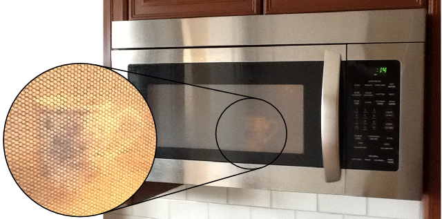
The engineers who design microwave ovens use this feature to let you see inside without getting your face cooked. Have you ever noticed that the window is a metal mesh with holes about a millimeter or two wide? Since these holes are much smaller than the microwave wavelength, it acts as a solid wall to the microwaves, but lets light pass through.
See HyperPhysics for more about the physics of microwave ovens.
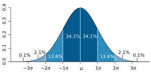
Gaussian distribution
[image
source]. The percentages indicate how much of the distribution
is within a given number of standard
deviations .
These are all applications of what is known as the Bandwidth
Theorem. The position resolution of a wave () and its wavelength resolution (
)
are approximately equal (
). By resolution, I mean the amount that the wave spreads
over positions and over wavelengths. The spread of a wave usually
doesn’t have clear-cut boundaries, and this complicates a general
statement of the theorem. However, if the distribution over space
has a Gaussian shape (see figure) with a standard deviation
of
, then the distribution of
wavelengths has the same standard deviation,
. (For the mathematically
inclined, this
web-based textbook has a nice derivation. It’s because the
Fourier Transformation of a Gaussian with standard
deviation
is another Gaussian with standard
deviation
.)
The Bandwidth Theorem is usually stated in terms of frequency (the
number of waves that pass per unit time, related to wavelength
as where
is the
speed of the waves) and time (the duration of a wave pulse is its
spatial extent divided by its speed,
). The theorem was used to identify an upper limit on the
number of telegraph clicks that can be transmitted through a wire,
or the number of bits that a computer can transmit by wi-fi, which
is essentially the same thing. If a bit is represented by a
Gaussian wave-pulse with standard deviation
, then the wave that carries it is spread over a Gaussian
distribution of frequencies
because
(a little algebra, the factors of
cancel).
A computer with
an 802.11b/g wi-fi
card transmits 54 million bits per second, which
is = 18.5 nanoseconds per bit. (Travelling
at the speed of light, each bit is about 18.2 feet long.) The
frequency spread is therefore
= 54 MHz around the nominal radio frequency of 2.4 GHz (a 2% spread).
Wireless routers switch channels to avoid overlaps between your home
network and your neighbor’s, but these channels are only about 5 MHz
apart (below).
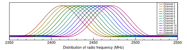
Distribution of radio signal strength (power) among radio frequencies for the 13 wi-fi channels used in the U.S. and Europe. These distributions are not quite Gaussian (they have side-lobes) because the bit pulses are not quite Gaussian (they are sharp square pulses).
Even on different channels, your data and your neighbor’s data interfere. Wireless routers can partly distinguish communications on different frequencies in much the same way that human brains distinguish red light and green light. However, most wireless routers are colorblind to channels that are very close to one another— in practice, at most three or four channels are distinguishable in any one location: channels 1, 6, and 11 in the U.S. and 1, 5, 9, and 13 in Europe. When there are too many wireless hotspots in the same spot, computers have to take turns downloading data. That’s why a busy coffeeshop has a slow Internet connection.
Newer wi-fi protocols like 802.11n transmit bits at much higher rates. Because they are faster, their signals occupy a broader range of frequencies, and thus fewer computers can be active at once. This can ironically lead to less total data transfer for a group of computers, so the protocols have fall-back modes to slow down the bit rate and open up more communications channels. The Bandwidth Theorem is as much a constraint on technology as the Second Law of Thermodynamics or the speed of light.
I first learned about the Bandwidth Theorem in quantum mechanics
class, since the Heisenberg Uncertainty Principle is a special case
of it. Fundamental particles such as electrons are wave-forms with
a range of spatial positions and speeds. The speed, or more
precisely, the momentum (velocity times mass) of an electron is
encoded in the wavelength of its wave as where
is the
wavelength,
is the momentum,
and
is a very
small fundamental
constant. Since the electron is a wave, the Bandwidth Theorem
applies and there is a relationship between its spatial
extent
and its momentum
distribution
:
The electron-wave is also interpreted as a probability distribution
because a measurement demanding an exact position will cause the
electron to pick one randomly, with probability in proportion to its
wave-form. That’s why this is called an Uncertainty
Principle, because the wave-like spread in its position could be
interpreted as an uncertainty in its position. That’s also why the
Principle has an inequality: the uncertainty will always be greater
than or equal to . The Bandwidth Theorem sets the
lower bound and any other sources of uncertainty can only increase
it.
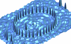
A quantum corral of cobalt atoms on a carbon surface, at extremely low temperatures so that the atoms don’t move much.
The fact that electrons are waves would be inconvenient if you
wanted to know their exact positions, but convenient if you want to
measure the shape of a very small thing. The wavelength of an
electron in an electron microscope,
= 2–12 picometers, is about 10 times smaller than a typical X-ray
microscope, and therefore sensitive to 10 times smaller things.
Also unlike electromagnetic waves, electrons are charged, so they
react more sensitively to a charged surface, such as the outer
electron clouds of a sheet of atoms.
It is therefore possible to take pictures of individual atoms. Exactly like the pictures of viruses (which are also taken with electron microscopes), they have no real color, but a shade of blue-grey usually conveys the etheralness of it. On the right is a picture of actual atoms, pushed into a “corral” by the tip of an electron microscope. (The repulsive force of the electrons’ charge can also be used as a manipulating device.) Inside the corral, the electron-wave surface ripples like water in a bucket: the shape of the boundary creates a resonance.
The non-spherical shapes of heavy nuclei make them more likely to split in nuclear reactions.
At even smaller scales, particle beams explore the shapes of nuclei and individual protons (three-quark structures) and mesons (two-quark structures). These experiments measure scattering angles and momentum transfer in collisions, which have an abstract relationship to the shapes of the particles that are collided or are briefly created in the collision. These shapes, known variously as structure functions, deep inelastic scattering, and parton distribution functions, are usually regarded as a means to an end: they are needed to predict the production rate of particles in collisions, so that you know whether you should have discovered that new particle yet or not.
My own thesis could be cast as a measurement of the size of an Upsilon meson. I was actually measuring the probability of Upsilon production in electron-positron collisions, but I couldn’t resist making a non-relativistic approximation and converting the number into a physical size. An Upsilon meson, which is an orbiting quark-antiquark pair, both of them b or “beauty” quarks, is a spherical cloud approximately 0.27 femtometers wide. This is about a billion times smaller than a virus, just as a virus is about a billion times smaller than us.